VLOOKUP function in Power BI

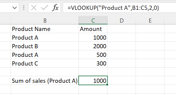
In Excel we use VLOOKUP when we need to find things in a Excel range by row:

Analog of Excel VLOOKUP function in Power BI is LOOKUPVALUE. Notice, that the function has its limitations.

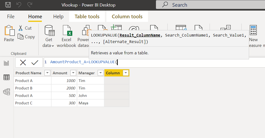
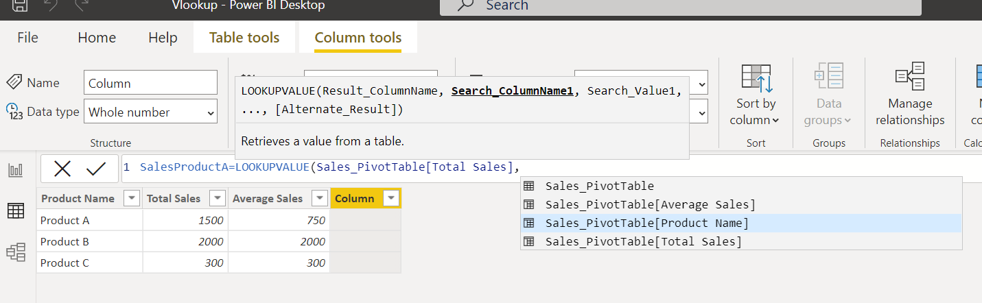
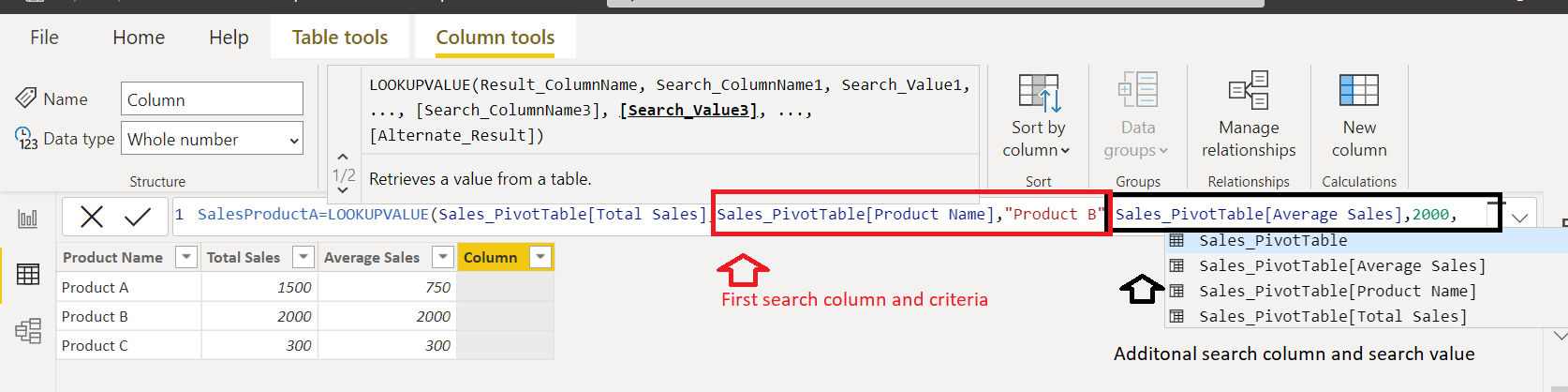
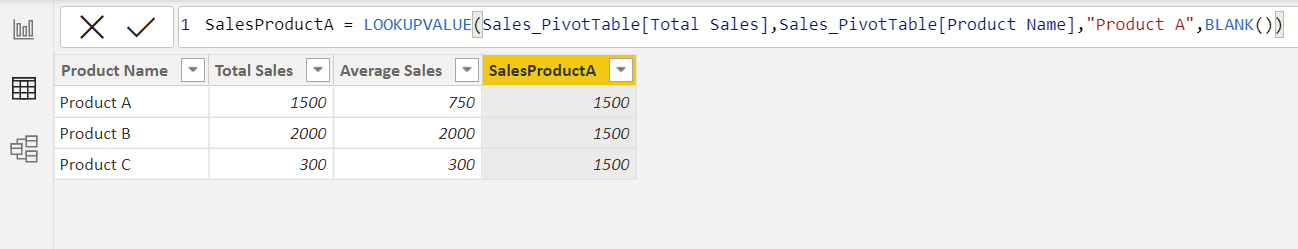
Syntax of this function actually is similar as in Excel but has its specificity. First argument is the name of column which contains the result (column "Amount"). When we assign the second argument - we specify area of the search. In our case this is column "Product Name", it contains information about key what we search. In our case - names of products:

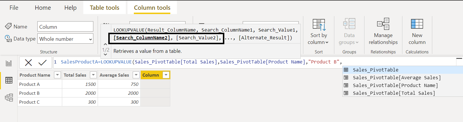
Note that in Power BI version of vlookup function we can specify addition search columns. In Excel such functionality we could achieve by concatenation of values of the target columns.

In LOOKUPVALUE function also we obligatory need to specify alternative value if LOOKUPVALUE return null.

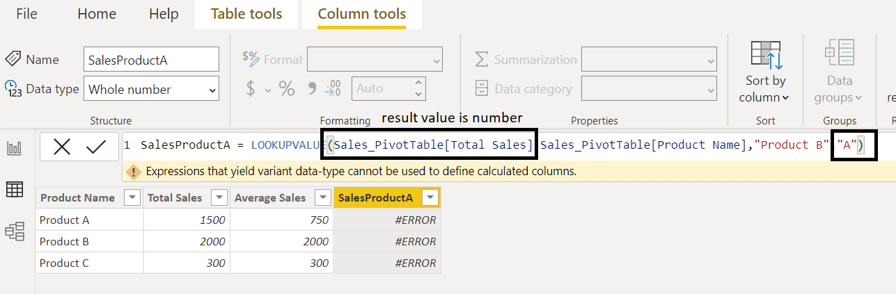
Please note that alternative result value should be the same type as value we search. Example of error when we estimate search value number and alternative value as text:

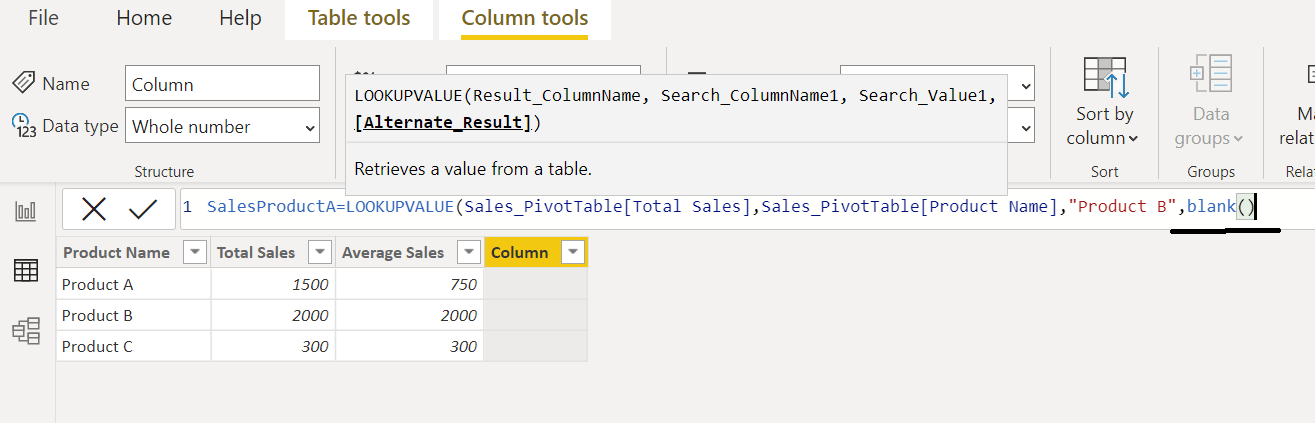
In this way we have two approaches: first one to use number, for example 0; second variant - use function BLANK():

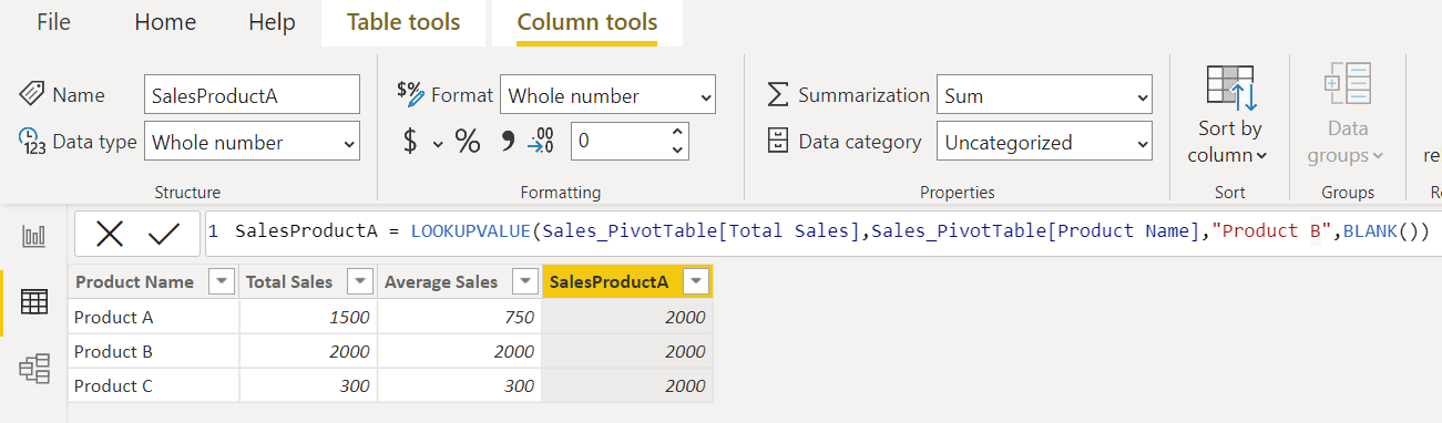
At the beginning of the article we show example of vlookup function in Excel. Our formula now returns total sales of Product B but not total sales of Product A. If we correct the formula, we obtain total sales of Product A - 1500.

LOOKUPVALUE in Power BI will not work in expected way if we have severel rows:

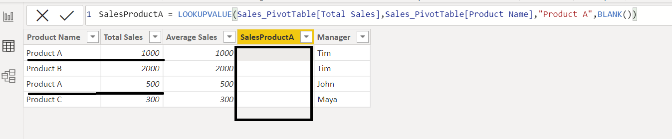
In Excel VLOOKUP will return first matched value (Product A - 1000) but in Power BI LOOKUPVALUE will return error. The reason of this because we have two values: Total Sales of Product A by Manager Tim (1000) and Total Sales of Product A by Manager John (500).

In this situation, when it is expected several values we have to use aggregation functions instead of LOOKUPVALUE function. In most cases, when we do analysis we know if we need max, min, average value of our "two values".

General algorithm:

1. we choose aggregation function;
2. we apply filter to source;
3. we apply additional functions to our result column.

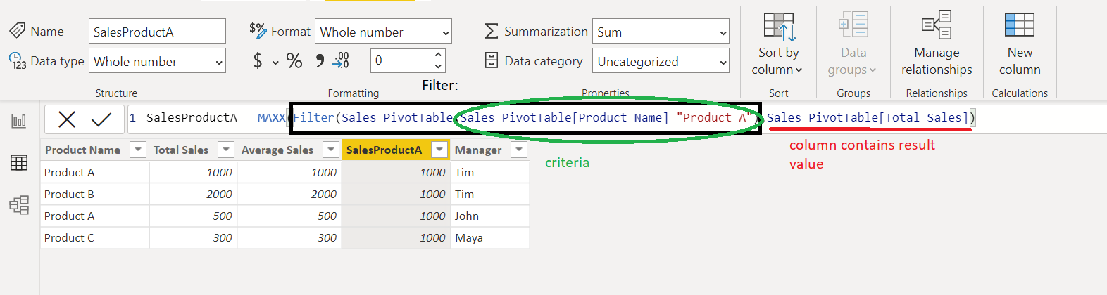
All aggregation formulas have the same structure: Aggregation Function(table,expression) Apply appropriate filters we can obtain result like VLOOKUP in Excel. In addition at result set we could obtain values that we get when create pivot table in Excel.

Example 1: If we want to obtain maximum Total Sales of Product A

1. We use function MAXX
2. We apply filter to table by Name of the product Filter(Sales_PivotTable,Sales_PivotTable[Product Name]="Product A")
3. We specify column which contains result values or expression.

Result: 1000 (Total Sales of Product A, Manager Tim)

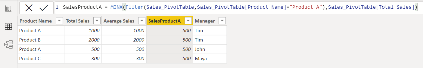
Example 2: If we want to obtain minimum Total Sales of Product A

Result: 500 (Total Sales of Product A, Manager John)

Example 3: If we want to obtain average Total Sales of Product A

Result: Average Total Sales of Product A is 750 = ((1000, Manager Tim)+(500, Manager John))/2

Other approach is to use function RELATED but we have restriction like in case of LOOKUPVALUE. The value that should be returned have to be single, in other cases we will obtain error. Also we have to make relation between our result table and our lookup table. Notice, that in this case we also obtain statistics by other products. In some cases this is not we need:

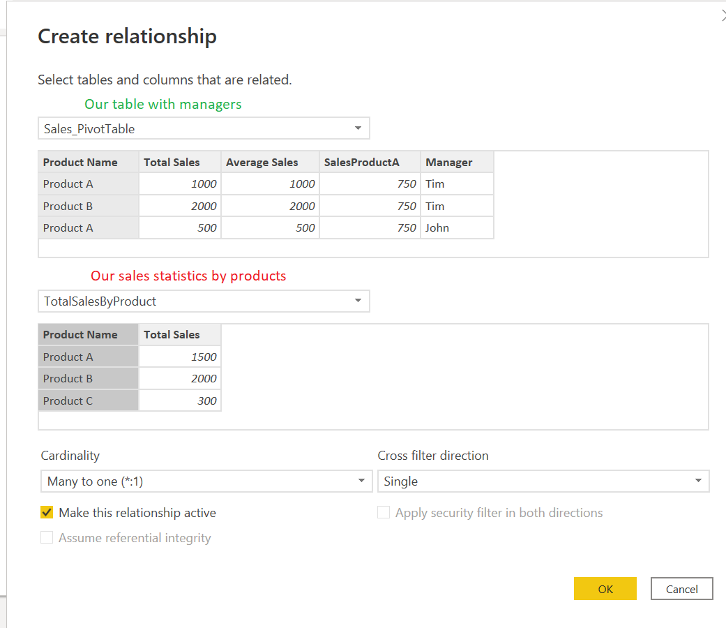
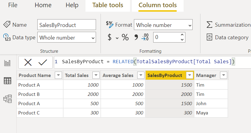
Function to obtain value from other table: RELATED(column) . Result function: SalesByProduct = RELATED(TotalSalesByProduct[Total Sales])

Summary

1. If we expect single value we could use functions LOOKUPVALUE and RELATED. Using function RELATED we are required the relation between tables. LOOKUPVALUE could be useful if we want repeat the same value by one criteria.
2. Aggregation functions (for example MAXX,MINX,AVERAGEX and ect.) do also additional calculations across ranges. They can be useful in complex calulations when you need obtain data ignoring current relations between two tables.